How to expert Digital Video Stabilization – Part 2

Ben Weiss – Imaging & Computer Vision Developer
Yury Schwarzman – Imaging & Computer Vision Team Leader

In our previous post, we took a look at some of the aspects that make video stabilization a must-have feature in many different camera applications. We then dove into the details of the first two stages of the stabilization process: feature detection and feature tracking/matching. In this post, we’ll describe motion model estimation (that is, the last stage of the motion estimation part) and go over the motion correction stages: motion smoothing, rolling shutter correction, and frame warping.

Motion model estimation

Three motion models will be mentioned here. Each model describes the scene or the camera movement with a different number of degrees of freedom (DOF). As the number of DOF increases, the motion estimation is more accurate and the overall stabilization process produces better results.

The translation model works only on the X and Y axes, that is, two DOF.
The similarity model describes translation in the X and Y directions, as well as uniform scale and rotation, giving a total of four DOF.
The homography model provides the most complete description of the scene transformation under 3-D camera motion, and has eight DOF.

As can be expected, to accurately estimate a transformation with more DOF, the system will need more data, which in turn will require more memory and generate a larger load on the processor. For an optimal trade-off between performance and processing load, we use the similarity model for motion smoothing. As we’ll see later, rolling shutter correction requires the homography model.

We use the RANdom SAmple Consensus (RANSAC) algorithm to estimate the frame-to-frame camera motion model from the pairs of features generated at the last step (feature tracking/matching). This algorithm is a well-known iterative method to fit a model to a set of observed data that contains outliers. In this context, the inliers are the pairs of features that represent the global motion (or the background motion), and the outliers are the remaining pairs representing the local motions and the measurement noise. We assume that the global motion can be estimated from the largest set of inliers (rolling shutter distortion is ignored at this stage).

To get an accurate estimation of the motion, the developer needs to ensure that the features are uniformly distributed over each frame. This can be achieved by tuning the detector and the tracker/matcher to be sensitive enough to give a valid response even for the features placed on low-textured areas of the frame.

Motion smoothing

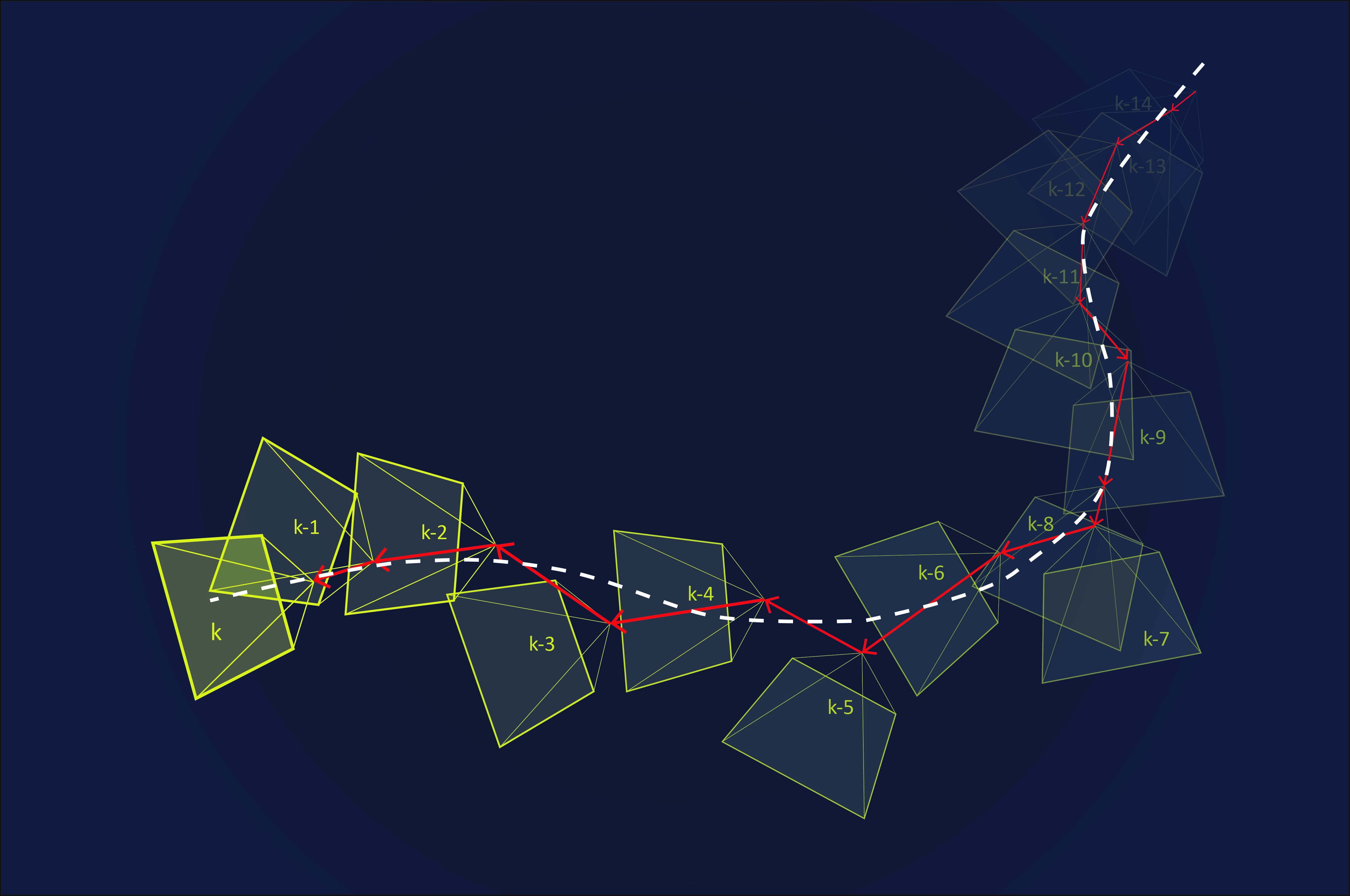
After the frame-to-frame motion model is created, the results are accumulated to create the estimated camera path. At this stage, the path will be noisy and include jitters. To smooth out the path, we use the Kalman filter. This algorithm filters out noise by using statistical inference and estimations of the joint probability distribution over the variables from a series of measurements. The algorithm is recursive, and works in two steps: prediction and update. For each measurement, a prediction is made based on the current state according to a given a state transition model. Then, according to the new measurement, the state is updated, while taking into account the uncertainty of the measurement. Each motion component is filtered separately: translation in X, translation in Y, scale, and rotation.

The accuracy of the smoothing stage strongly depends on how well the Kalman filter is configured according to the anticipated noise characteristics and the preferred smoothed path. The three main parameters to be tuned are the state transition model, the covariance of the process noise, and the covariance of the observation noise.

For the first one, we use a constant velocity model: the state of each component (X, Y, Scale, and Rotation) includes position and velocity values. On each step, the position is predicted only by using the previous position and velocity. For the process and observation noise covariance matrices, we tune both of them for a specific motion and noise type. Shooting video while walking, driving a car, or from a drone device produces different types of motion and motion noise (jitter) with a different frequency distribution. By studying many different types of motion and noise, we have been able to generate parameters that render excellent results and provide a sleek viewing experience.

Figure 2. Illustration of camera movement over time. Motion smoothing takes the frame-to-frame motion model (represented by the red arrows) and filters out the noise to generate a smooth motion path (represented by the white dashed line).

Rolling shutter correction

Currently, the most prevalent technology for capturing digital images is CMOS image sensing. CMOS image sensors capture the image by exposing and reading-out one pixel line at a time. The result of this method is that the captured image is distorted if motion occurred while the whole image was being scanned. This motion might be due to the movement of the camera, the scene, or both. This phenomenon is known as the “rolling shutter” effect, or rolling shutter distortion. In digital video, low-frequency motion will generate either a stretch or a skew distortion, while high-frequency motion will generate a wobble, commonly known as the “jello effect”.

In our method, the first step in correcting this distortion is to split the frame into horizontal strips. For each strip, the homography model is estimated. The next step is to ensure the boundary conditions across the vertical direction by spatial interpolation of the homography model parameters.

Frame warping

The last stage of the stabilization process is frame warping. In this stage, part of the image will be cropped according to a predefined region of interest (ROI). The ROI can also be selected dynamically depending on the motion magnitude. Larger motions will require more aggressive cropping. Typically, about 10% of the margin in each direction will be lost to cropping. To maximize the ability to correct unwanted motions, it is a good idea to keep the ROI as close as possible to the center of the frame.

There are three relevant warping models:

The affine model is sufficient for stabilization and correction of rolling shutter distortion caused by slow motion. The results of this model are decent but sub-optimal. To achieve more accurate results, a more complex model is needed.
The homography model gives very good results for both stabilization and slow-motion rolling shutter. However, when dealing with high-speed rolling shutter (such as vibrations from a drone motor), a more complex model is again needed.
In the map model, each pixel in the output frame is explicitly mapped to a pixel in the input frame. This model is the most computationally intensive, but it delivers the most accurate results and handles rolling shutter caused by all types or motion. In this model, the lens distortion correction can be incorporated at the same stage without additional processing.

Lessons learned about video stabilization

As we have seen, video stabilization is a complex problem, with many stages and parameters. Each stage can be approached with various methods, each one featuring different advantages and disadvantages. One of the important things about this process is that it contains many tradeoffs: performance versus power consumption, quality versus computation time, high-frequency or low-frequency motion targeting, and so on. Because of this, only the specific application of the stabilization software can determine the best methods for the process. Even so, here are some concrete conclusions that we have reached:

Use a rich test set: When developing a software video stabilization solution, it is important to have a rich test set that covers various motion types.
RANSAC isn’t perfect: While RANSAC is a very powerful technique, it has its shortcomings. Spatial image coverage at feature detection and tracking/matching stages is very important for accurate motion estimation.
Feature matching is superior: The second stage of motion estimation can be performed by either feature tracking or feature matching. While each method has its pros and cons, our experience has taught us that, in general, feature matching is superior to feature tracking in terms of accuracy and robustness.
Both fixed-point and floating-point are needed: While fixed-point accuracy is sufficient for the feature tracking stage, floating-point accuracy is required for motion model estimation and smoothing.
Smoothing is significant: The motion smoothing algorithm, while having a relatively low complexity, makes a significant contribution to the overall quality.
Homography gets best results: The less complex models can be calculated faster, with less memory and power, but a homography motion model is required to achieve the best visual results.
Frame warping requires the most computation: The most computationally intensive part of the whole process is the frame warping stage. The performance of the entire video stabilization algorithm is usually dominated by this stage.

Find out more about CEVA’s DVS solutions by clicking here.

#Digital Video Stabilization #DVS #EIS #OIS #Optical Image Stabilization

Deep Learning Imaging & vision Sensor fusion

Video Stabilization Using Computer Vision: Tips and Insights from CEVA’s experts

May 10, 2016

Imaging & vision

Digital Video Stabilization: Smooth Footage Without Expensive Mechanics

February 3, 2016