

6 min read
Not too long ago, we had a series on Robot Dead Reckoning. However, believe it or not, there’s more still to say. Today, we’re going to go into finer detail about the type of testing we do to show you how deep the rabbit hole can go. Jump in with me, won’t you?
For newer readers, I’m going to review a few quick concepts. If you’re a veteran of the space, feel free to skip ahead to Testing Robot Dead Reckoning Performance.
A Quick Review of Robot Dead ReckoningSLAM
What is Robot Dead Reckoning?
By fusing data from multiple sensors, dead reckoning creates an estimation of location using measurements of speed and direction over time. Just like with people, the robot may not know exactly where it is, but it has a strong estimate. It may also be referred to as odometry.
What sensors are used?
Robot dead reckoning algorithms generally use wheel encoders, an IMU, and optical flow sensors (like the one in your mouse). Some optical flow sensors for robotics have both LED and LASER light sources which work better on rough and smooth surfaces, respectively. Robot odometry can also be calculated using the IMU and either of the other sensors alone.
Why is this helpful?
Some robots use camera- or LIDAR-based simultaneous localization and mapping (SLAM) algorithms to determine where they are and better clean. Robot dead reckoning provides crucial speed and direction information that’s part of this algorithm. Other robots do not need to build a persistent map (they just need to return home when they are done their job), and they may be able to get by with dead reckoning alone.
Note: This is the Cliffnotes/Sparknotes version of the basics to understand the rest of this post.
Testing Robot Odometry Performance
Collecting Data
I promised a deep dive, so let’s get started by going over how we tested our algorithms. We previously collected data in a mock-home environment based on an international specification. However, in order to log more testing data directly tied to dead reckoning accuracy, we tested in a simpler and smaller environment with more changes in direction. These more frequent changes incorporated in the following driving algorithm:
- Drive forward at 0.3 m/s until a wall is impacted
- Stop for 0.1 s
- Drive backwards at 0.2 m/s for 0.5 seconds
- Rotate a random value between 45° and 180° at 0.6 radians/s
- The direction of rotation is selected such that the robot heading is within 720° of its original heading
- Every 60 seconds, remain stationary for 5 seconds
Our test subject was a robot development platform from one of the leading manufacturers of consumer robots in the world. This gave us a strong comparison point for what the most successful companies were doing. This test robot had its own odometry algorithm outputs which we logged, in addition to the RAW data and output of our own MotionEngine Scout rider module.
With both sets of data, we still needed a truth measurement. For this, infrared cameras were positioned to cover the testing space and keep track of the robot’s position. The data from these cameras was used as truth. These same cameras can be used for all sorts of high accuracy, low latency projects, including this bow that auto-aims.
The last variable we wanted to tweak in our testing was different types of surfaces. For these tests, we ran the robot over hardwood, low pile carpet, high pile carpet, faux-tile, and combinations of these surfaces. These surfaces introduce error with their relevant sensors, but we’ll go more in detail on that later.
Now that we have test data collected, a truth to compare it to, and a number of different test surfaces to run it on, the last piece we need is a metric to determine accuracy. Comparing error based on start and end positions makes the most sense for a metric as we are measuring positional performance. This trajectory error can be broken down in a few different ways.
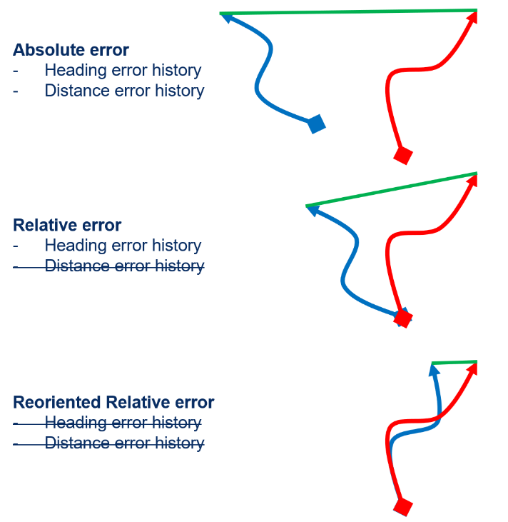
Absolute error is just the difference between where the robot thinks it is and where it really is. This is easy to understand, but the absolute error at any point in time depends on the history of heading and distance errors at all previous points in time, so it is hard to generalize this metric.
With relative error, we zero out the positions to match at the start of the measurement period to eliminate the effect of previous distance errors. Reoriented relative error also removes the effect of previous heading errors. This final metric can be computed over many fixed-size windows in the trial, giving us a continuous view of the error growth rate per unit distance travelled.
Reoriented relative error is less intuitive than absolute error, but is more generalizable to the variation in driving patterns and mission durations in the home robotics use case.
In order to get a full view of how error grows throughout the course of a trial, we calculated reoriented relative error over a sliding window of data based on a set distance traveled (1 meter). In other words, we calculate the relative error of the algorithms over every 1 meter window of distance traveled, sliding the window by 1 centimeter for each data point.
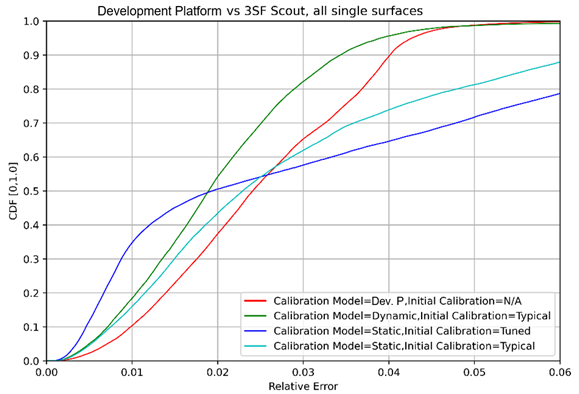
This plot shows the distribution of these error values for each surface and algorithm used in a CDF (Cumulative Distribution Function) as seen in the example above. Looking at the plot (lines to the left are better), we can easily compare the median performance vs the worst case or other percentile and identify outliers. From this, you can see that across all surfaces, a dynamic calibration model with a typical initial calibration leads to consistently better performance than the development platform.
Optimizing Robot Odometry Performance
What do these calibration models mean? Why do we care about calibrating sensors?
Well, dear reader, let’s start with the higher-level question. We care about calibrating sensors because even though sensors are quality controlled to be within a certain specification listed on the datasheet, each individual sensor varies. This is where dynamic calibration comes into play. In short, each sensors behavior varies enough to influence overall accuracy and adjusting for these differences maximizes performance.
As you may have guessed from this, a static calibration model uses an initial calibration and sticks with it. However, a dynamic calibration model uses IMU and wheel measurements to adjust the optical flow sensor’s output. This maintains accuracy over time, through temperature changes, wheel slips, surface reflection changes, variation in surface softness, and more.
The various flooring types we tested on matter, as optical flow sensors and wheels can react differently depending on what they’re driving over/on. Wheels can slip on surfaces and give inaccurate readings on the wheel encoder. Optical flow sensors work better on some surfaces than others, and careful calibration increases their accuracy. The way you use the sensor also matters. Leading optical flow sensors for robotics include both an LED mode (illuminating the floor texture for tracking) and a LASER mode (inducing a “speckle pattern” that can be tracked). Identifying when to switch modes and when to keep the one you have is critical to getting the best performance possible.
Through our meticulous and exhaustive testing of flooring surfaces, we’ve determined typical calibration values for each optical flow light mode. The scale of each needs to be adjusted based on the flooring type. With dynamic calibration, IMU data can help adjust the initial calibration in real time during operation.
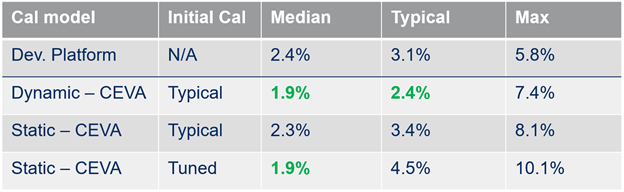
The Tuned calibration method in our analysis represents the upper limit of calibration accuracy. It’s calculated by passing the raw sensor data through our algorithms offline, and adjusting the optical flow sensor scale such that the error is as close to 0 as possible.
The results of our analysis show that we’re over 22% more accurate than a market leader over the variety of surfaces tested with the most realistic calibration mode you would see in a robot (dynamic, typical).
This post was intended to highlight our testing and analytical capabilities, and hopefully pique your interest for more details. If it was successful, please contact us for more information on what MotionEngine Scout can do for your robotics projects, and keep an eye out for an upcoming white paper showing detailing more specifics of our testing and analysis.
Ceva